Plamen Kolev

Genetic Programming

Revised justification

As the first biologically inspired machine learning algorithm, I decided to use Genetic Programming. Genetic Programming is suitable for classifying multiple classes. An Oxford journal about classifying microarray datasets talks about ways GP can be used to classify and diagnose particular types of cancer (Kun-Hong L. et al. 2008). An implementation of a Genetic Programming for classification works by applying divide and conquer strategies to the training data, splitting it into multiple sets of decision trees. The leaves of the trees represent different classes (Jeroen Eggermont et al. 2004).

In the original proposal, I make the case for using Genetic Algorithm with k-nearest neighbours, but later decided to not use it, as GP frameworks such as epochx contain all the necessary libraries and tuning strategies that will provide a better result with the ability to do more fine-grain tuning. It will also allow me to explore a more generic solution.

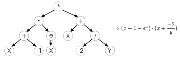
In genetic programming, each decision branch is formed by a mathematical expression (functions). For the dataset, I experimented with different ‘syntax’ functions. The findings are documented in the tuning section for this algorithm, but the most effective were the trigonometric ones.

Description of implementation

As mentioned above, I used the epochx library framework to bootstrap my implementation. I created a new source package called GP, which contains GPClassifier.java, GPControl.java and GPWrapper.java. The implementation of the GPControl class is very similar to the provided sample one, as its purpose is to test the actual implementation. Minor modifications were made to accommodate for the newly created data structures. Another modification is exposing the generateSubSolution to return GPClassifier, as this class is used in the main method to write performance and configuration statistics to a report file called gpstats.csv.

The GPClassifier class contains a genetic program instance that has learned on the training data and implements classifyInstance and printClassifier. Those methods are passed to the underlying genetic programming class GPWrapper, the class is acting as a middle man between the control and the genetic programming class.

The GPWrapper class contains all the necessary constructs and tunable variables for the epoch framework,which are described in the tuning section.

GPWrapper.java constructor.

``` java syntax.add(new SignumFunction()); syntax.add(new SineFunction()); syntax.add(new CosineFunction()); syntax.add(new ArcTangentFunction()); syntax.add(new AbsoluteFunction());

syntax.add(new AddFunction()); syntax.add(new DivisionProtectedFunction()); syntax.add(new SubtractFunction()); … for (int i = 0; i < Attributes.getNumAttributes(); i++) { syntax.add( variables[i] = new Variable(“dim” + i, Double.class) ); } ```

The constructor allows for an arbitrary attributes to be passed as the syntax, but the syntax functions are specially tuned for the given dataset, as trigonometric functions are suitable for classifying the circular representation of the data.

An auxiliary function called parseData is provided just to store the data in an internal array for later usage.
This class also returns itself as an instance when generateClassifier is called. The method is responsible for setting the different tuning parameters and training the genetic program.

GPWrapper.java classifyInstance method.

java public int classifyInstance(Instance ins){ GPCandidateProgram a = (GPCandidateProgram) this.getProgramSelector().getProgram(); for (int i = 0; i < Attributes.getNumAttributes(); i++) { this.variables[i].setValue(ins.getRealAttribute(i)); } Double result = (Double) a.evaluate(); return (int) Math.round(result); }

The classifyInstance method is used after the GP is trained to determine the class of the data (black or white).It uses the GPCandidateProgram object with the best fitness (closest to 0). That program is given the instance attributes and evaluates a solution. The output is an integer that represents the class.

As the GPWrapper extends from the epochx’s GPModel, it also implements getfitness method. This method is applied to each member of the population (candidate program). Each candidate produces an output when given the input data points from the training set. If the output of the program matches the class (predicts it), a score variable is incremented. The best candidate program should have a score which should be as close to the size of the training set as possible.

printClassifier simply finds the fittest program from the candidate pool and prints its representation, which is just a string of nested functions.

Similar to the NeuralClassifier, this class also contains setconfig function, which allows for environmental variables to be set and used to tune different parameters. Finally, the classifier also implements visualise, which draws a representation of the training and test data to the screen using Jpanel in a class called Picasso.

Tuning for the provided dataset

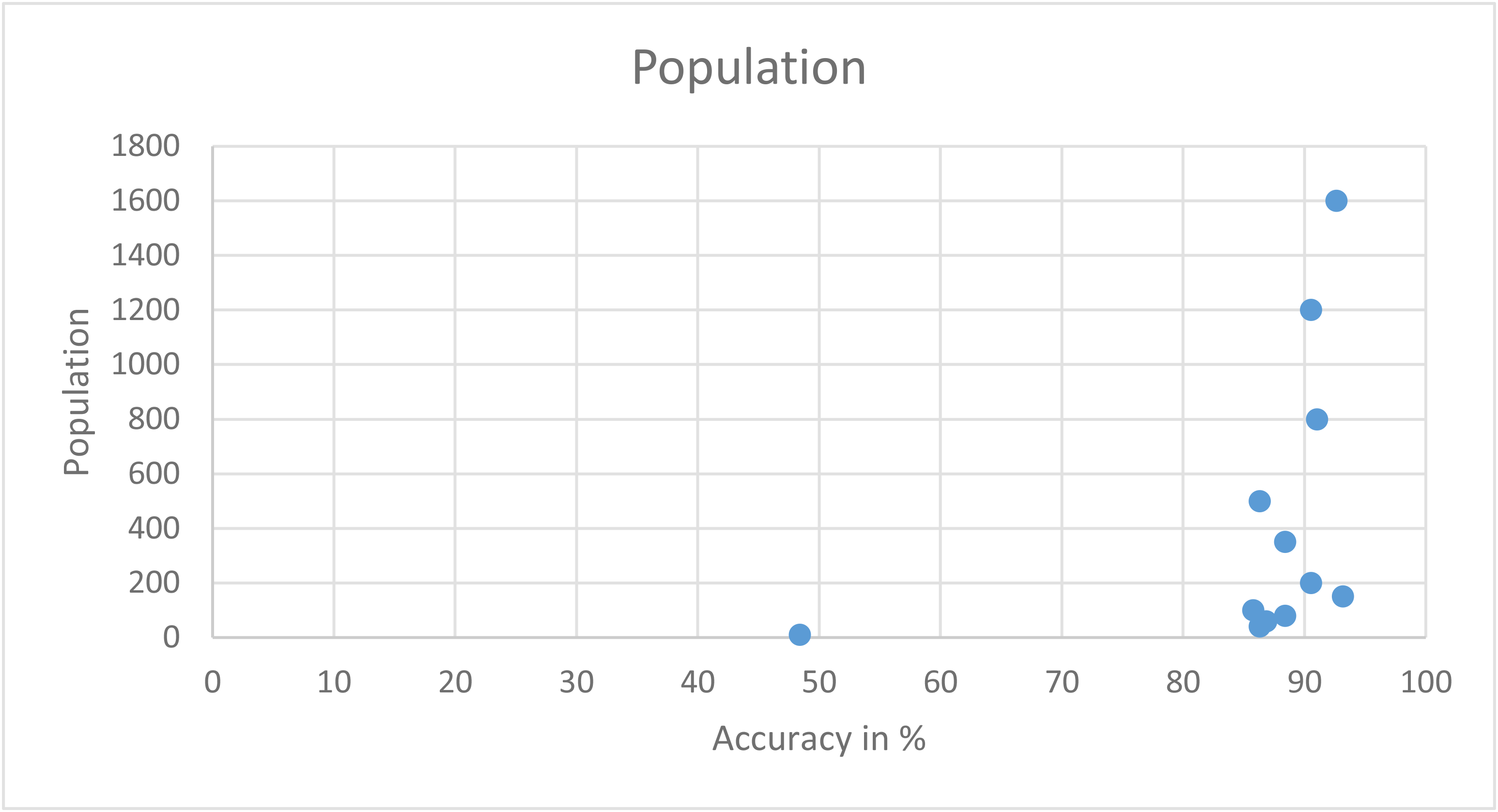
For the tuning, I exposed a variety of parameters that are used when creating and training the classifier. The most important tunable parameter is the population size, which represents the number of generated random program candidates. A large population range between 600 - 1200 members provided enough diversity to generate the most efficient classifiers and below 600, the accuracy relied mainly on the random seed value and luck, making the predictions unreliable.

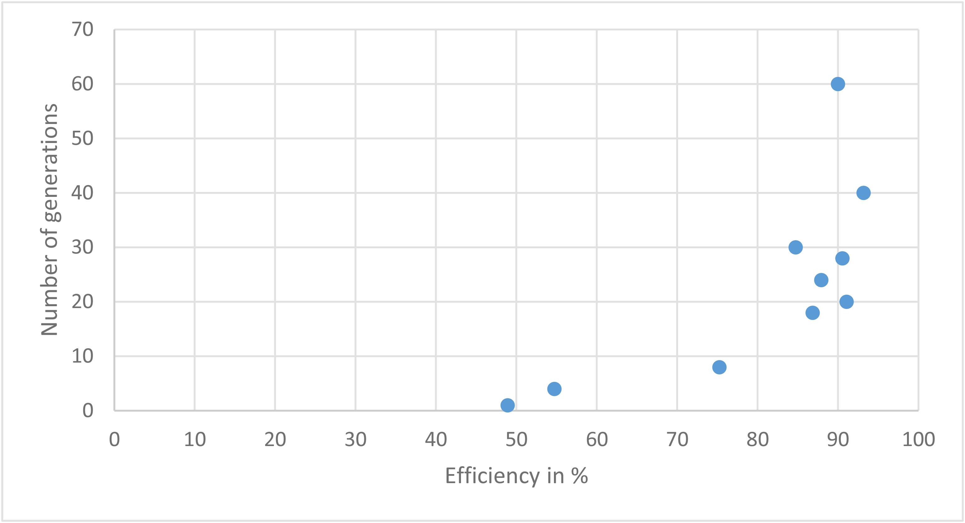
I also decided to experiment with the generation size. When a large generation set is configured, at some point the population diversity evens out and the fittest individual does not change much. A value between 20-70 generations is the most appropriate, as it gives the programs enough time to evolve and mutate, but keeps the running time short.

Another important factor in the efficiency was selecting the syntax functions when creating the program trees. They had very significant impact on the evaluation time and efficiency.The performance of each function varied, as some were very beneficial, some had not much impact and others had a negative effect . The implementation does not include flags for tuning which type of function to use, but rather includes a selection of the the most effective ones. The highest result I was able to achieve is using SignumFunction as well as the trigonometry functions. I included division, subtraction and addition, as they helped with the program’s diversity.

Experimenting with number of selected elite members, crossover, mutation and reproduction probability did not provide a significant difference during my experiments.

Performance report

Runtime	Efficiency in %	Population size
0.506	48.421052631578945	10
7.528	86.31578947368422	40
10.396	88.42105263157895	80
30.763	90.52631578947368	200
53.695	86.31578947368422	500
163.121	90.52631578947368	1200
232.42	92.63157894736842	1600

GP algorithm with different population size

Time	Efficiency in %	Generation number
1.087	48.91304347826087	1
1.267	54.736842105263165	4
2.045	75.26315789473685	8
3.582	86.8421052631579	18
12.429	91.05263157894737	20
10.704	87.89473684210526	24
17.317	90.52631578947368	28
16.921	84.73684210526315	30
14.252	93.15789473684211	40
25.816	90.0	60

Table showing runs with different generations (stopping criteria)

I also experimented with different crossover probability, number of elite chromosomes and mutation but they did not improve or lower the efficiency. The difference I noticed is the runtime, as these parameters allow the GP to perform additional operations pore often. I have included a table with my findings for completeness.

Time	Efficiency %	Elite population count
22.11	92.63157894736842	1
38.558	93.15789473684211	4
42.268	90.0	12
34.73	97.89473684210527	18
43.304	88.94736842105263	24
35.337	96.3157894736842	30

Table of different size of the elite population

Time	Efficiency in %	Crossover probability
77.397	90.0	0.1
87.546	94.21052631578948	0.3
82.201	87.36842105263159	0.4
58.289	93.15789473684211	0.8
62.03	94.21052631578948	1.0

Table of different crossover probability

Time	Efficiency in %	Mutation probability
15.015	85.78947368421052	0.1
94.777	89.47368421052632	0.2
79.374	88.94736842105263	0.4
105.695	93.6842105263158	0.6
62.391	88.42105263157895	0.8
71.862	91.57894736842105	1.0

Mutation probability

Neural Network

Revised Justification

As mentioned in the coursework proposal, I chose Neural network as the method for classification for several reasons: It is suitable for classifying multiple ‘features’ as neural networks have been widely used for speech recognition, facial recognition and malignant cancer detection (Álvarez L. et al. 2009). The Universal approximation theorem also states that a neural network has the ability to can compute every function. Yoshua Bengio and Yann LeCun also mention in their paper that neural networks do not have limitations in the efficiency of the representation of certain types of functions as compared to other approaches.

I also wanted to use a neural network, as it is a very exciting and hot topic in computing and wanted to experiment with the different activation functions and parameters.

Implementation description

Implementing the solution was a multi-part process. During my research, I found it suitable to use Neuroph java framework for the supervised neural network. I then outlined key features and functions that need to be implemented, tuned and integrated. The following is a detailed description of them.

Firstly, I created a special package called Neural, which contains the main class Control.java of the application and the NeuralClassifier.java class witch is a wrapper for Neuroph. For the code of Control.java, I used most of the sample code provided (time keeping, printing training and test data, etc.) with some minor modifications. I also replaced the Wrapper classifier with the neural implementation file NeuralClassifier.java. The new main class was also modified to allow for stats dumps to csv file used to generate statistics for the report.

My NeuralClassifier.java extends from the Classifier class and thus implements classifyInstance and printClassifier. Its purpose is to be a middle man between the given framework and Neuroph. Because Neuroph uses its own data representation for the training and testing sets, an auxiliary function is provided as part of the implementation called instanceSetToDataSet which parses the InstanceSet and converts it to DataSet used by Neuroph.

NeuralClassifier.java function instanceSetToDataSet.

java public DataSet instanceSetToDataSet(InstanceSet trainingData){ int dataRows = Attributes.getNumAttributes(); DataSet td = new DataSet(dataRows, 1); ... // Data normalisation code skipped // Data scaling code skipped td.addRow(new DataSetRow(inputs, new double[]{instance.getClassValue()})); } ... }

Here, the TrainingSet is converted to Data set with dynamic rows. This function is used in the constructor to bootstrap the MultiLayerPerceptron.

Constructing the actual class is done in the following way:

NeuralClassifier.java function constructor.

java NeuralClassifier(InstanceSet trainingSet){ ... this.initConfig(); DataSet trainingData = this.instanceSetToDataSet(trainingSet); this.mlp = new MultiLayerPerceptron(ACTIVATION_FUNCTION, Attributes.getNumAttributes(), HIDDENNODES, 1); BackPropagation b = (BackPropagation) mlp.getLearningRule(); b.setMaxIterations(ITERATIONS); b.setMaxError(MAXERROR); b.setLearningRate(LEARNINGRATE); ... this.mlp.learn(trainingData); }

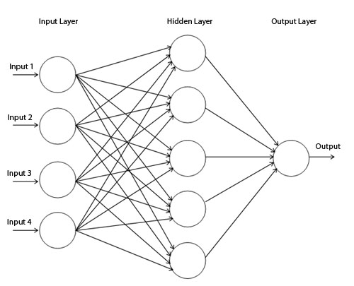
As mentioned in the proposal, I am using Multilayer perceptron with back-propagation, the above function creates and configures the neural network instance. As described in the lecture notes, the MultilayerPerceptron uses an activation function which is one of the parameters for tuning, I have set the Sigmoid Transfer function as the default as the highest results are often achieved using it, but others are explored as part of the performance report. For the input layer, I use as many neurons as data attributes in the training set, allowing for a generic solution when applying different datasets.

Neuroph has a construct that allows for the tuning of extra parameters, like the number of iterations, max errors and learning rate, they are also configured and demonstrated in the performance section. The given Attributes, InstanceSet and Instance classes were used throughout, as they provided helpful methods give the necessary information to make the solution generic. When going though the source code, I also noticed that some examples were scaling and normalising the data, so I decided to include these features into the implementation. I used DecimalScaleNormalizer.java function normalizeScale example from the source directory of neuroph to optionally scale down each data point by a factor of 10 based on a flag. This function and the flag normalise in instanceSetToDataSet function are extra tunable parameters that I experimented with but found to cause harm to both the performance and the efficiency.

NeuralClassifier.java function classifyInstance.

``` java public int classifyInstance(Instance ins) { // provide the classifier with the inputs int numattrs = Attributes.getNumAttributes(); double[] attributes = new double[numattrs]; for (int i = 0; i < numattrs; i++) { attributes[i] = ins.getRealAttribute(i); } this.mlp.setInput(attributes);

// calculate neural network output
this.mlp.calculate();
double[] result = this.mlp.getOutput();
int prediction = (int) Math.round(result[0]);
if(prediction > Attributes.getNumAttributes() || prediction < 0){
    return -1;
}
return prediction; } ```

classifyInstance function is used to return a prediction after the network has gone through the learning process. In this case, the MultiLayerPerceptron is given the instance data , after which the probability for each class is computed and returned. The prediction is 0 for black, 1 for white and -1 if it goes outside the domain range, or more generally, between 0 to n-1 where n is the class range.

NeuralClassifier.java function printClassifier.

java public void printClassifier() { for (Double weight : mlp.getWeights()) { System.out.print("Output weights: " + weight); } System.out.println(); }

For printing the final classifier, I grab the weight of each node in the neural network and print it out.

Finally, I created a helper function called initConfig() to read environment variables that allow for dynamic tuning and shell execution of the solution for generating statistics. I have included the shell scripts used for generating the performance data under “gp_shell” for the genetic programming algorithm and “neural_shell” for the neural network algorithm. They have been developed and tested under Ubuntu 16.04 and work by using environmental variables. When running the program, it will create a report file in the current directory with the performance, duration and the tuned parameters.

Finally, the classifier also implements visualise, which draws a representation of the training and test data to the screen using Jpanel in a class called Picasso.
# Description of adjustment and tuning
A neural network allows for a variety of parameter tweaking and different optimisations.
Reading up on different approaches for training a neural network, The report (Moriera, M 1995) describes the purpose of a learning rate. The paper suggests to use a learning rate that is sufficiently large to allow for the learning process but small enough to guarantee effectiveness. For that purpose, I used the learning rule function setLearningRate(value) and found out that a very small value in the range of 0.01-0.1 usually yields the best results. I experimented with more than one hidden layers, but often the result was identical or slightly worse but it increased the learning time, sometimes by a factor of two. Hence I decided to ignore the tuning of multiple layers, and instead allow for the tuning of different hidden nodes in the single layer. Just one layer is used, because the data to classify is not complex enough to benefit from it (not many features). Tuning the learning rate had a significant impact on the accuracy and I found that a lower learning late had a very positive impact on the correctness of the classifier for a very small performance cost.

Neuroph also provides couple of activation functions as part of the MultilayerPerceptron package. Experimenting with them, I thought initially that the gaussian function will yield the best result, but by far the most efficient function was sigmoid, which consistently achieves results above 90% accuracy. To contrast that with the tanH function, it has an extremely negative effect on the accuracy, making the prediction absolutely wrong. Another function that performed very poorly is the linear function, which yields 50% accuracy, making the classifier more similar to a coin toss.

An article on standardising data for neural networks (McCaffrey J. 2014) an argument for normalisation of the data is made. I have allowed for a normalisation flag in my implementation, but enabling it has a negative effect due to the data being evenly distributed and relatively short. As mentioned above, data can also be scaled, but again, this also has a negative effect on the accuracy.

Performance report

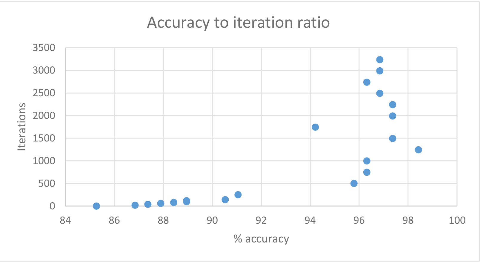
Time in seconds	Efficiency in %	Number of iterations
0.189	85.26315789473684	1
0.489	86.8421052631579	20
0.838	87.36842105263159	40
1.121	87.89473684210526	60
1.371	88.42105263157895	80
1.642	88.94736842105263	100
10.2	96.3157894736842	748
13.524	96.3157894736842	997
26.391	97.36842105263158	1993
28.076	97.36842105263158	2242
21.338	96.84210526315789	2989
32.731	96.84210526315789	3238

Efficiency with different iterations

The table above shows improvement in performance with the increase of iterations. In my case, it peaked at about 1500-2000 iterations, at which point it did not have a significant impact on the efficiency but it impacted the running time.

Time	Accuracy in %	Hidden nodes
6.379	82.10526315789474	1
9.108	84.21052631578947	3
12.434	91.05263157894737	6
12.125	94.21052631578948	10
14.309	98.42105263157895	17
16.069	97.36842105263158	23
15.644	98.42105263157895	24
17.264	95.78947368421052	29
17.871	97.89473684210527	33
18.304	97.36842105263158	36
20.96	97.36842105263158	40

Impact on different hidden nodes

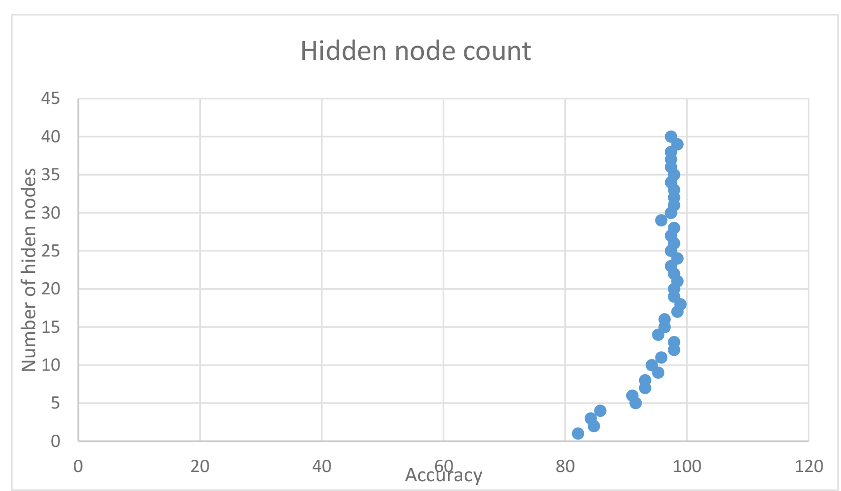
In this case, increasing the amount of hidden nodes had a significant impact on the accuracy, with it peaking at about 17-24 nodes. I found that using 18 hidden nodes fairly reliably produced around 98% accuracy, thus chose it as the base for some runs.

To keep this report short, I will include a graph of learning rate and max error results without including the tables, but the data can be found and viewed under neuralstats.csv

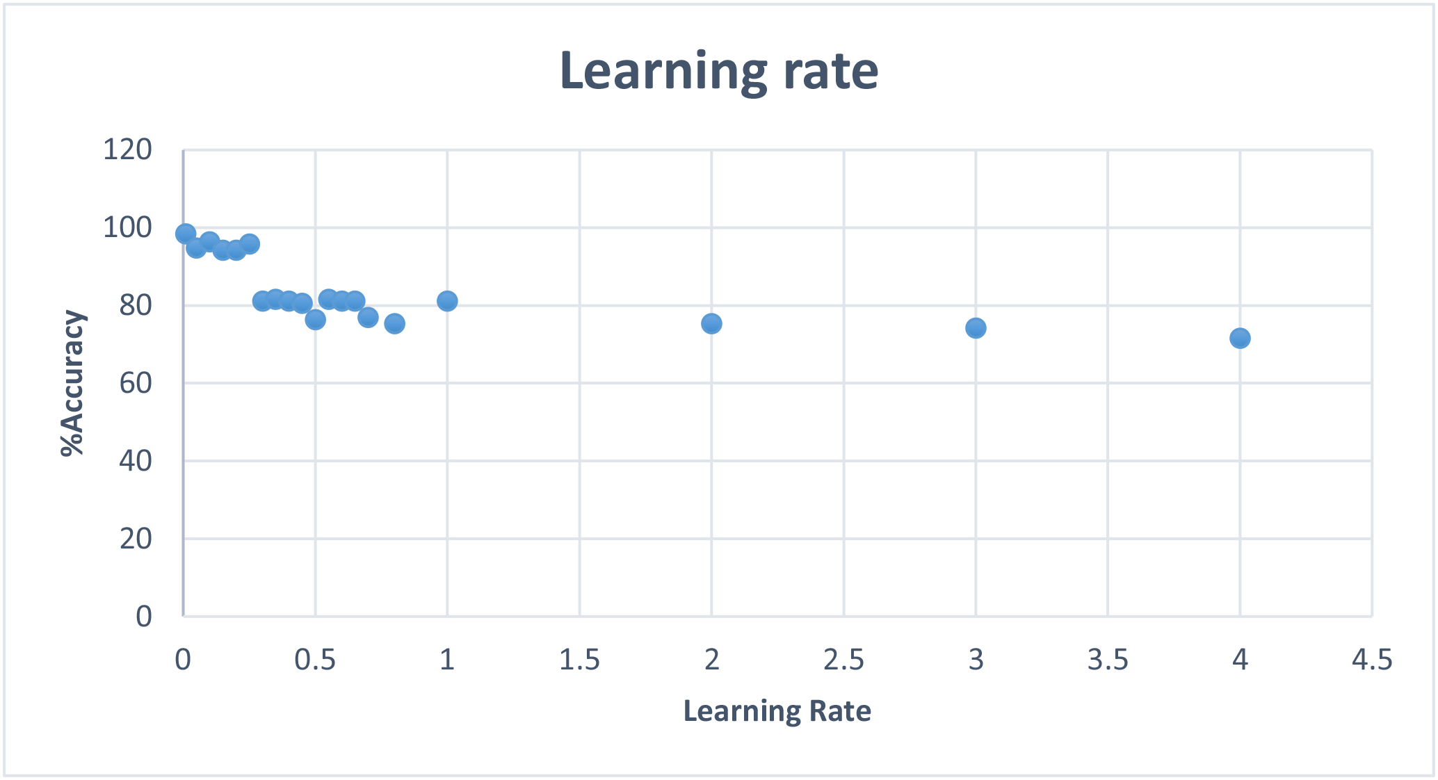
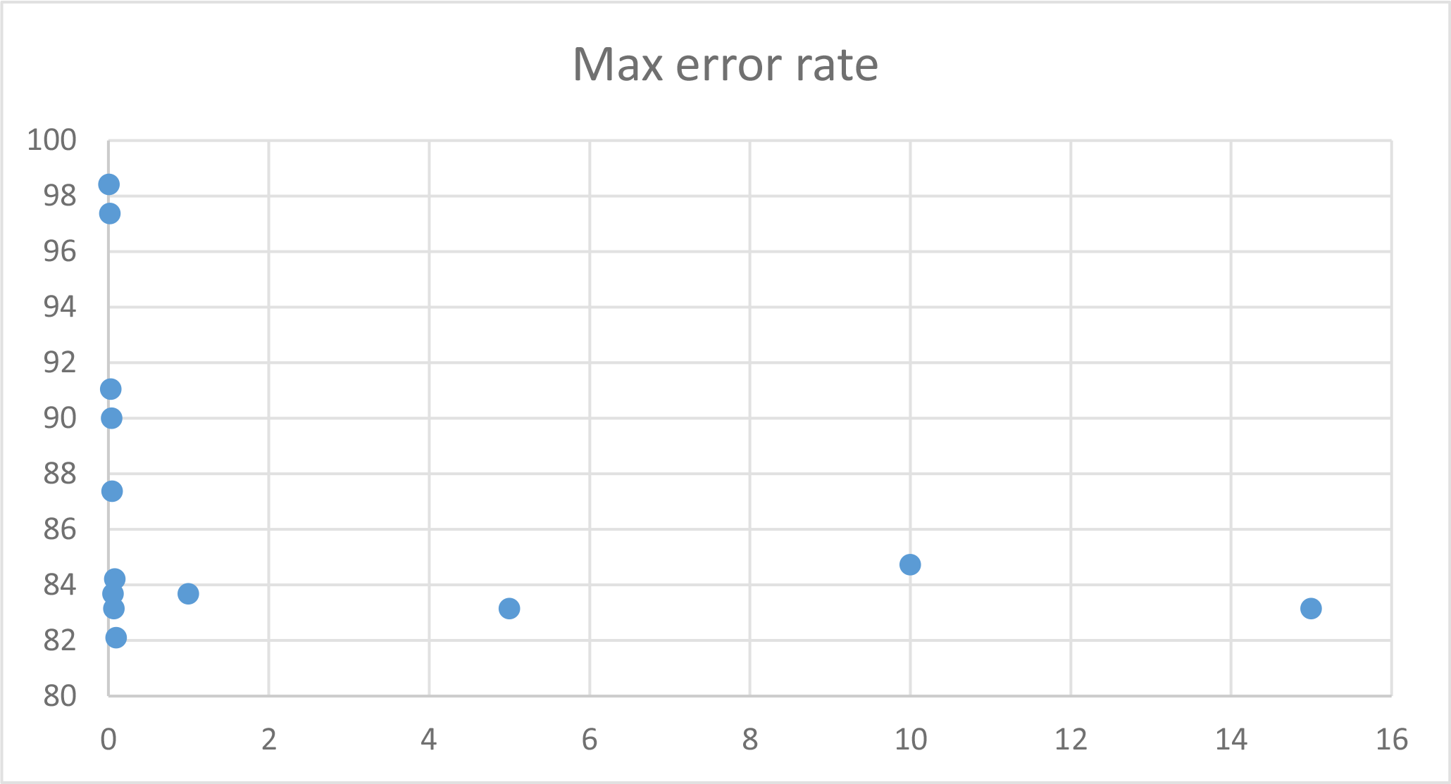
I observed that learning rate and max error rate were the most efficient at around 1% and increasing them had mostly negative effect on the effectiveness.

Time	Efficiency in %	Normalised
15.487,	82.63157894736842	yes
15.009	98.42105263157895	No

Normalisation vs. no normalisation

Time	Efficiency in %	Scaled down
15.652,	74.21052631578947	Yes
15.705,	96.3157894736842	No

Down scaling (factor of 10) vs. no down scaling

As mentioned above, experimenting with scaling or normalising the data did not yield a positive effect, on the contrary, it reduced the classifier’s ability to make accurate predictions.

Time	Efficiency in %	Activation function
16.638	95.78947368421052	SIGMOID
16.37	92.63157894736842	GAUSSIAN
14.283	50.0	LINEAR
13.596	17.20430107526882	TANH
14.101,	50.0	TRAPEZOID

Different activation functions

Comparison between methods

The difference between genetic programming and neural networks (MLP) was very noticeable. The neural network produced a more generic solution, as less knowledge was provided to it. To contrast that with the GP, many variables had to be tuned specifically to achieve the optimal result using syntax functions that are relevant to the solution. Neural networks are also faster and more efficient, outperforming the GP implementation. The implementation of the neural network is also a bit harder to reason with and the library hides most of the complexity away from the developer.

On the other hand, the Genetic Programming algorithm seemed more simple and intuitive, the tunable parameters had a direct impact on the result and the classification representation is simple. The program is also less generic as it required special tuning to achieve good results. It also does not provide consistent accuracy, where as the Neural Network had much smaller margin of error.

General note

The sourcecode folder contains gp_shell and neural_shell bash scripts that will work only on linux.

To manually run the java executable, use the following commands
java -cp CSC3423.jar Biocomputing.Neural.Control dataset/Training.arff dataset/Test.arff
java -cp CSC3423.jar Biocomputing.GP.GPControl dataset/Training.arff dataset/Test.arff
Where CSC3423.jar is the executable jar file in the out folder and the arff files are the Training and Testing data sets.
The Neural network accepts the following environmental variables: ITERATIONS, GENERATIONS,ACTIVATION_FUNCTION, HIDDENNODES,MAXERROR,LEARNINGRATE,NORMALISE,SCALE.
GPClassifier environmental varialbes: POPULATION_SIZE, GENERATIONS, ELITES, CROSSOVER_PROB, MUTATION_PROB, REPRODUCTION_PROB and TOURNAMENT_SIZE.
In windows, one can use the command set HIDDENNODES=5 followed by the java run command to set these values.

References

1. Moreira, M. (1995). Neural Networks with Adaptive Learning Rate and Momentum Terms. Available at https://infoscience.epfl.ch/record/82307/files/95-04.pdf. Accessed on 12.12.2016

2. Kun-Hong L. et al. (2008). A genetic programming-based approach to the classification of multiclass microarray datasets. Available at http://bioinformatics.oxfordjournals.org/content/25/3/331.full. Accessed on 14.12.2016

3. McCaffrey J. (2014). How To Standardize Data for Neural Networks. Available at https://visualstudiomagazine.com/articles/2014/01/01/how-to-standardize-data-for-neural-networks.aspx. Accessed on 14.12.2016.

4. Jeroen Eggermont et al (2004). Genetic Programming for Data Classification: Partitioning the Search Space. Available at http://liacs.leidenuniv.nl/~kosterswa/SAC2003final.pdf. Accessed on 15.12.2016

5. Álvarez L. et al. (2009). Artificial neural networks applied to cancer detection in a breast screening programme. Available at http://ac.els-cdn.com/S0895717710001378/1-s2.0-S0895717710001378-main.pdf?_tid=c4a6e3c0-c2b3-11e6-9ddd-00000aab0f6b&acdnat=1481798983_5428dbaa26e2d27c669d7906a5c1a77a. Accessed on 15.12.2016

6. Bengio Y., LeCun Y. (2007) Scaling Learning Algorithms towards AI. Available at http://yann.lecun.com/exdb/publis/pdf/bengio-lecun-07.pdf (Accessed: 16 Nov 2016).

Credits

1. Genetic programming tree image taken from http://www.ra.cs.uni-tuebingen.de/software/JCell/images/docbook/gp.png

2. Multilayer perceptron with back-propagation image taken from https://www.codeproject.com/KB/dotnet/predictor/network.jpg